You’ve probably seen a convolution before, whether you know it or not. And they’re super useful in deep learning.
\(\text{Convoluti}\!\ast \!\text{ns}\)
Let’s say we have two polynomials \(P(x)\) and \(Q(x)\) what is their product. Now you may recall the FOIL or BOX method from gradeschool. Lets define these polynomials as
\[P(x) = \sum_{i=0}^{m}{a_{i}x^{i}, \:\:\: \text{and}\:\:\: Q(x) = \sum_{j=0}^{n}{b_{j}x^{j}}}\]Now these definitions may look scary but I encourage you to write down some degree polynomial lets say 2 and expand the summation from 0 to 2 to prove the above to yourself. Let \(R(x) = P(x)Q(x)\). What is the summation for \(R(x)\)? It is:
\[R(x) = \sum_{k=0}^{m+n}{c_kx^k}, \:\:\: \text{where } c_k= \sum_{i=0}^{k}{a_ib_{k-i}}\]And so it turns out that \(c_k\) is a discrete convolution of the coefficients. To see this better we can extended the bounds of the summation to the infinites (we can do this because all the terms outside the original range are zero):
\[c_k= \sum_{i=-\infty}^{\infty}{a_ib_{k-i}}\]which is exactly the formula for a discrete convolution. You might see it like
\[(a \ast b)[k] := \sum_{i=-\infty}^{\infty} a[i]b[k-i]\]Some quick notes on notation: the \(\ast\) symbol means convolution. The number/variable inside the brackets is the index for the corresponding sequence (Ex: \(a_i= a[i]\)). And \(:=\) is read “defined as”.
The formula for a convolution on continuous functions is the following
\[(f \ast g)(s) := \int_{-\infty}^{\infty} f(x) g(s - x) dx\]where \(f(x)\) is the kernel and \(g(x)\) is the function to be convolved. Again this looks pretty similar to the discrete convolution, we switch to integration to catch all those values between the integers (non integers) as it makes it much easier than a summation.
\(\text{Applications}\)
You can’t talk about convolutions without taking about signal processing as its one of convolutions most known applications (at least before CNNs became popular).
\(\text{Signal Processing}\)
Before I start I would just like to say I’m not to familiar with signal processing so forgive me for any mistakes I make. So according to Wikipedia signal processing is the analysis of signals like radiowaves, images, sound, and more.
According to Steven W. Smith in his The Scientist and Engineer’s Guide to Digital Signal Processing convolutions are the “single most important technique in Digital Signal Processing” (See I told they were important). The first two algorithms you learn in Digital Signal Processing (DSP) involving convolution are the input and output side algorithms.
Essentially, the input side convolves each input with the impulse response to produce the output signal or \(x[n] \ast h[n] = y[n]\). It does this by decomposing the input signal into versions of the input signal and then convolves each with the impulse response and then synthesizes all the versions to get one output signal.
The output side algorithm is the same thing except we go from the output’s perspective (it looks at what inputs we need to get a particular output). If you didn’t understand that don’t worry. If you would like to learn more about convolutions and DSP check out Smith’s book.
\(\text{Probability}\)
Let’s say we have two dice. Each dice will have a separate probability distribution. If we want to find out what is the probability that both die sum to some number we need to be able to combine the probability distributions. We do this through convolutions (in this case the new combined distribution who show how likely each sum is).
I will give an overview of what this would look like for discrete random variables (SideQuest: Try to find out how convolutions work for continuous random variables), but first some terminology (This is only for review purposes). We say \(X\) is a discrete random variable if its values can be counted, otherwise, \(X\) is a continuous random variable. The range or support of \(X\) (denoted \(R_X\))contains all the possible values of \(X\) aka \(R_X = \{x_1, x_2, x_3, ...\}\). The probability mass function (PMF) of \(X\) is the function \(p_X(x_k) = p(X=x_k), \:\:\:\text{for} \:\:\: k =1,2,3,...\). And for all countable values (\(\forall x \in\) ):
\[\begin{equation} p_X(x) = \left\{ \begin{array}{l l} p(X=x) & \quad \text{if } x \in R_X\\ 0 & \quad \text{otherwise} \end{array} \right. \end{equation}\]Let \(X\) be a discrete random variable with range \(R_X\) and PMF \(p_X(x)\). Let \(Y\) be another discrete random variable with range \(R_Y\) and PMF \(p_Y(y)\).
The PMF of \(Z\) such that \(Z = X + Y\)
\[\begin{align*} p_Z(z) = \sum_{y=R_Y}{p_Y(y)p_X(z-y)} \\ p_Z(z) = \sum_{x=R_X}{p_X(x)p_Y(z-x)} \end{align*}\]They both give us the same solution since \(Y+X = X+Y\). In the first equation we loop over the possible values of Y and we find the probability that \(X = z-y\). The second one is the same but the places of the variables are swapped.
Now about the sidequest I mentioned before make sure to take a look at probability density functions.
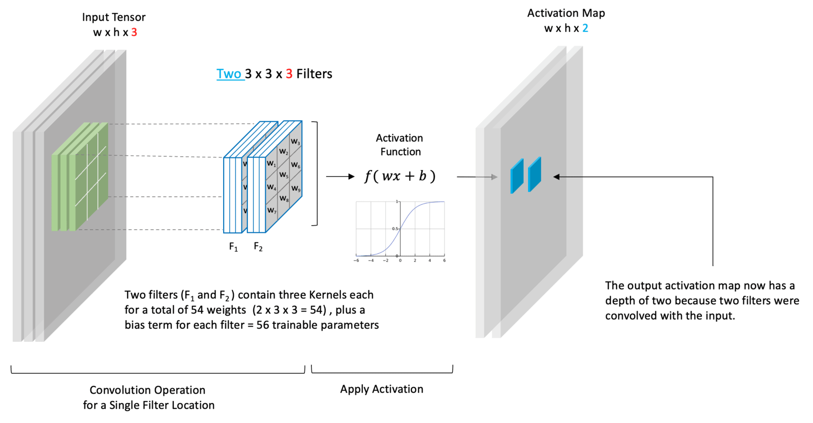
\(\text{CNNs}\)
CNNs are where most people (nowadays) encounter convolutions and there’s a lot to them so I’ll be posting it in a part 2.
\(\text{References}\)
- Overlay image courtesy LearnOpenCV
- The scientist and engineer’s guide to digital signal processing Steven W. Smith, ISBN:978-0-9660176-3-2
- Taboga, Marco (2021). “Convolutions”, Lectures on probability theory and mathematical statistics. Kindle Direct Publishing. Online appendix. Website Link